Measuring a Classifier at Scale: LLM Labels, Human Review

The problem: a number nobody trusted

I have been working on a production classifier with three labels. The real domain does not matter here, so picture a toy sorter instead:

• a rubber duck is the common case;
• a Rubik’s cube is a smaller middle band;
• a colourful ball is rare, and it is the label that triggers automatic actions.

The system combines deterministic signals with an LLM-based classifier, and it returns one label per item.

We had a quality figure. It came from a frozen test set, and nobody believed it. The set was old and clean, and it did not look like the traffic the system was actually handling.

What we needed was a number measured on production data. We did not have a labelling team to produce ground truth at that volume.

This post is about how I got there. It started as a one-off investigation and ended as a small scheduled pipeline.

The short answer

• Label a stratified sample with an LLM that never sees the system’s answer. Its evidence has to match what the system saw, with the prediction removed.
• Replay the system offline and prove it reproduces every production prediction before you blame any signal for an error. Only then are counterfactuals (“remove this signal, does the label change?”) worth anything.
• Treat the metric as a survey, not a test run. Reweight by stratum, use stratified confidence intervals, and refuse to publish when a stratum loses too many labels.

Step 1: a labeller that cannot copy the answer

The first pass was manual. I took a short production window and gave the evidence to several LLM sub-agents working in parallel. Each one saw only the item and the signals, never the system’s label.

That second part is harder than it sounds. When the work later became a pipeline, a review found several separate ways the answer was leaking into the labeller’s input. Some were obvious, like a field whose value was the final label. Others were not: round-robin packing had encoded the stratum in each item’s position inside a batch record, so items are now shuffled with the run’s seed.

The fix that made this stick was structural. Signal fields reach the labeller through an allowlist, not a denylist. A test walks the signal registry, so a new signal breaks CI until someone decides what it is allowed to reveal. A denylist fails open: the next new field just gets through.

Step 2: reconstruct before you attribute

The first results did not match what the frozen set suggested, which is exactly why a measurement on real traffic was worth building.

The obvious next step is to count which signals appear most often in the errors. That is misleading, because signals co-occur. An item flagged by three signals will show up under all three, and counting says nothing about which one actually changed the label.

So I rebuilt the system’s decision logic offline from the real code, and checked it before anything else. The replay had to reproduce every production label in the sample, with no exceptions. It did. Without that, no attribution is worth reading.

With a faithful replay, I removed each signal in turn to see which labels flipped. Then I ranked the signals with a greedy set cover.

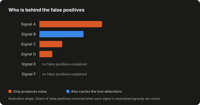
The chart shows the shape, not our numbers. Two lessons came out of it.

Errors concentrate. A handful of signals explained almost all the false positives. Most signals explained none.

The ranking alone is dangerous. One of the top signals also carried every true detection of the rare label. Removing it would have killed recall. Another one was pure noise and safe to fix. Frequency cannot tell those two apart; the counterfactual can.

Reading the raw data behind the noisy signals then showed why they fired, which is what turns a ranking into a fix.

One more habit: audit the labels too. One apparent miss turned out to be a labelling error. The item looked like a clear colourful ball, but in context it was not, and the system had been right.

Step 3: make it repeatable without fooling yourself

A manual investigation is useful once. The next step was a scheduled run on a batch inference API, orchestrated by the task queue.

Sampling

Strata are “predicted label × whether any signal fired”. Two combinations are structurally empty, since the system cannot predict a cube or a ball without a signal, so four strata remain.

Traffic is very skewed. I sample the same fixed number of items from every stratum, so the rare label is heavily oversampled on purpose.

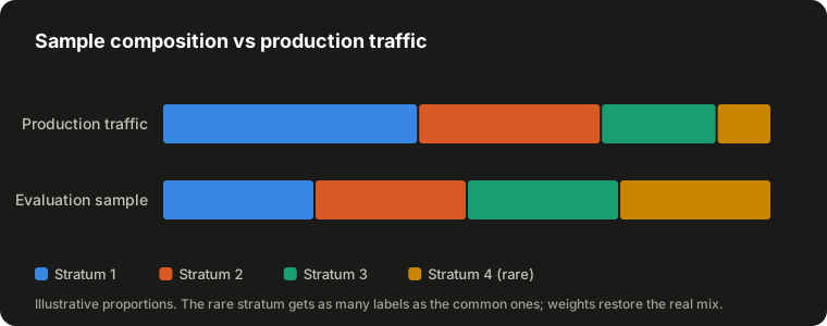
This means raw accuracy on the sample describes traffic that does not exist. Each stratum is reweighted by N_h / n_h, where n_h is the number of labels that actually came back, not the number planned.

Intervals

A binomial interval over the whole sample is wrong for a reweighted estimate. The variance of a stratified estimator is the weighted sum of the per-stratum variances.

The finite population correction also matters. In the rare stratum the sample is a noticeable share of the whole population, and ignoring that makes the interval look worse than it is.

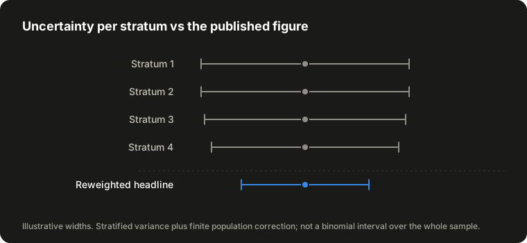
Each stratum on its own has a wide interval. The headline is narrower, because most of the weight sits in large, well-sampled strata. Both are reported: the headline interval next to the headline, the per-stratum intervals next to the per-class figures.

Losses are not random

LLMs refuse some content, and refusals correlate with the class you care about most. Measured on another model, refusals were many times more frequent in the rare stratum than in the common ones.

Losing those items leaves an easier sample, and precision goes up without anything failing. So coverage is gated per stratum:

• below a minimum, the run does not publish;
• below a higher threshold, it publishes with a warning.

There is deliberately no global threshold. A healthy global coverage can hide the loss of half the rare stratum.

Headline definition

A false positive is “predicted ball, labelled not ball”, because the ball is the label that acts. Accuracy is never published without macro-F1 next to it. With three unbalanced classes, accuracy goes up just by getting the ducks right.

Comparability

Each run stores a short hash of the rubric, the model, the reasoning effort and the evidence format. A change in any of them starts a new series, and the report says so.

The stratum weights are left out of the hash on purpose. A change in traffic mix is what the series exists to show, not a break in it.

Details that each produce a plausible wrong number

• Thinking blocks. A good share of batch records returned a reasoning block before the text. Reading content[0] silently drops them.
• Output order. Batch output does not come back in input order. Labels are matched by record id and by the item id the model echoes back, and some did come back misplaced.
• Missing records. Losses are found by set difference against the input, not by listing known failure symptoms. Listing symptoms only catches the ones you have already seen.
• Idempotency. Some SDKs fill an omitted idempotency token with a random UUID. Under a task queue with late acknowledgement, a retried task would then submit a second paid job. The token has to be derived from the run.
• Hashing sets. A Python frozenset iterates in a different order in each process, so the same set gave different digests on different workers. Tests were green; production would have split the series. Serialize canonically before hashing.

The unit tests needed the same suspicion. One fixture drew labels in the same proportions as its population, so raw counts matched the weighted shares by coincidence. Deleting the reweighting from macro-F1 left every test green.

Mutation testing found several surviving mutants like that one, and none of them was visible by reading the tests.

Step 4: a human in the loop

The pipeline gives you a number and a list of disagreements. It cannot say who was right in each one. That call needs a person, and a person needs a place to look.

So the last piece is a read-only review dashboard over the results. Nothing on it can be edited: every row is evidence behind a published figure, and a dashboard that could change it would quietly change the figure too.

It has three levels:

• Runs. One row per scheduled run, with its time window, its state, and how many labels came back per stratum.
• Metrics. The published figures for each run, with the full confusion matrix, the per-stratum numbers and the losses by cause. Anyone who questions the headline can check exactly where it came from.
• Items. Every labelled item of every run. This is where the review actually happens.

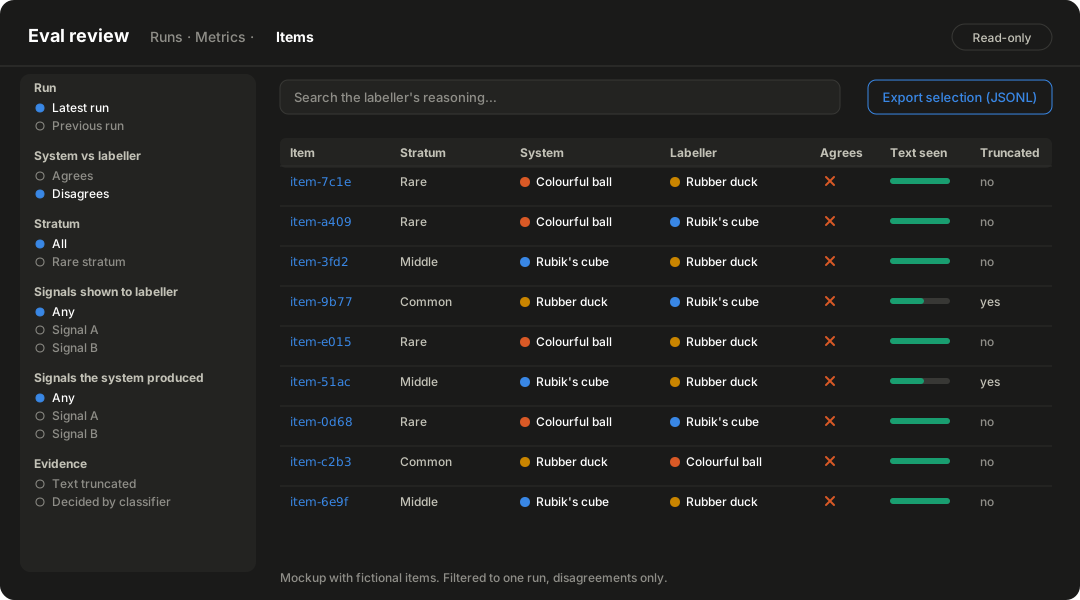
Filters that match the questions

The item list is built around the questions a reviewer really asks:

• Agrees / disagrees. This is the most useful filter. It compares two columns of the same row, the system’s label and the labeller’s, and it cuts a run down to the few items where the accuracy is actually lost.
• Run and stratum. Every review starts by pinning one run. From there you can go to, say, the rare stratum only.
• Which signals fired. There are two separate filters here: the signals the labeller was shown, and the signals the system actually produced. They are not the same list, because some signals are withheld and some are cut to fit the size budget.
• Evidence quality. Whether the item’s text was truncated.

The choices in those filters come from the system’s signal registry, not from the data. That includes signals no run has produced yet. Building them from the data would cost a query on every page load. Worse, it could hide old rows that carry a signal the current rules no longer show.

The labeller’s written reasoning is searchable as free text. In practice, that is how a disputed case gets found at all: you remember what the model said, not the item’s id.

One item, both sides

The detail page shows the two labels side by side, the labeller’s reasoning, and exactly what the labeller was shown: whether the text was truncated and how much of it was visible. The truncation flag alone is misleading. Long items are the ones that get truncated, so a truncated item often shows more text than a short one that was not.

The system’s label on this page is a copy taken when the item was labelled, not a live lookup. If the item is reprocessed later, the published figure and the rows behind it still agree.

From there, one link opens the full item as the system saw it. That is deliberately more than the labeller saw. The link says so explicitly, because it is an easy trap:

• a disagreement has to be explained from what the labeller was shown;
• a rule change has to be argued from what the system acted on.

For questions the dashboard cannot answer

The design principle was simple: fixed views answer the questions we already know, and an export answers the rest. Any filtered selection can be exported as JSONL and analysed in a notebook.

It is JSONL rather than CSV on purpose. Several fields are free text that people outside the team can influence. Making that text safe for a spreadsheet means changing the values, and the changes would land exactly on the unusual rows worth studying. JSON keeps them byte for byte, and keeps lists as real arrays.

The export stays on the analyst’s machine. What gets shared is conclusions, not files.

Each reviewed disagreement also adds to the human-adjudicated set that rubric tuning needs (see the limits below). The review is the thing that produces it.

Trade-offs and limits

• Agreement is not correctness. The pipeline measures agreement between two judges. When they disagree, the number does not say which one is wrong.
• Don’t tune the rubric against agreement. Editing the rubric until agreement goes up can simply teach the labeller to copy the system. Tuning needs a small human-adjudicated set, drawn from the disagreement bands and judged by domain experts rather than engineers.
• Correlated judges. When part of the system is itself an LLM reading the same content, two models agreeing is weaker evidence than it looks. Human review of disagreements is the real safeguard.
• Small base. Few runs so far. The method is sound; the conclusions are still early.

Conclusion

The valuable part of this work was not the labeller. It was the checks around it:

• a replay that matches production before any attribution;
• evidence that cannot leak the answer;
• intervals that respect the sampling design;
• a gate that refuses to publish a biased number;
• a dashboard where a person can study every disagreement in depth.

An LLM makes labelling affordable. Whether the result can be trusted still comes down to ordinary statistics and some discipline.